Deep Autoencoder Neural Networks for Maximal Christmas Decoration Enjoyment

My wife loves decorations. From Valentines Day to Easter to Thanksgiving, our house is adorned with interesting festive items. Her favorite season by far is Christmas. Every December we drive around trying to find the best Christmas lights. Inevitably, there are a few houses with lights that blink with the music, something I’ve always been fascinated with.
Two years ago I embarked on a mission to build my own Christmas Light Show, specifically this is what I had in mind:

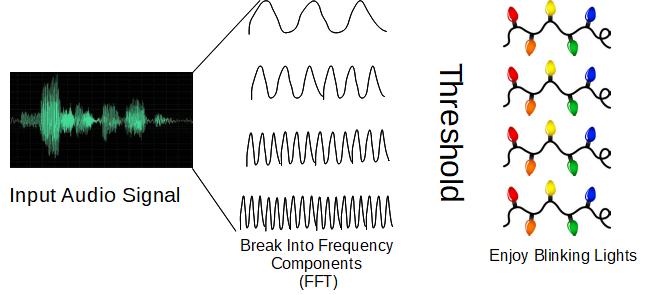
1. Break music up into even sized chunks
   
2. Convert each chunk into frequency components using FFT
   
3. Bucketize frequencies into the number of light channels
   
4. Activate a light channel when the decibels reached a certain threshold:
   

A brief Google investigation revealed I had been (thankfully) beaten to the chase. The open source lightshowpi project already had a full pipeline, took like 10 minutes to set up, and already had the FFT parallelized on the Raspberry Pi GPU (so you can apply it to streaming music!). Here is a video of our light show the first year (Christmas tree only):

What I’ve found over the past few years is that while the light show is certainly entertaining (After every song, every year, my kids have a deep expression of joy and clap and congratulate me on my show), I’ve been interested in ways to capture more of the structure of the sound in the blinking lights. The light blinking can be sporadic (especially during very fast parts of the song), and vocals are not always captured very well across vocal range.

Enter: Deep Autoencoder Neural Networks

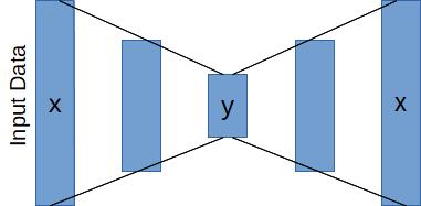
Autoencoders are intuitive networks that have a simple premise: reconstruct an input from an output while learning a compressed representation of the data. This is accomplished by squeezing the network in the middle, forcing the network to compress x inputs into y intermediate outputs, where x>>y. Here is a nice blog post from the Keras blog that goes into some detail on autoencoders for the mnist dataset.

So what exactly are we going to squeeze? Once you’ve processed the signal through the FFT, you can make a spectrogram (check out this super psyched YouTube video)… Time is on the x-axis, frequency is on the y, and the color represents the amplitude for that time/frequency. If you had a tuning fork tuned for a pure A4 note you’d have a solid (in this case red) line at 440Hz. The song we’ll study for the rest of the post is “A Mad Russian’s Christmas” by The Trans Siberian Orchestra, check out the spectrogram:

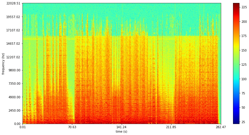
I encourage you to look at the spectrogram while you listen to the song, see if you can pick out the different sections. You’ll also notice why our simple heuristic method (frequency buckets + thresholding) doesn’t do a great job capturing the structure of the song. If you look closely at the spectrogram you notice characteristic bands representing the complex sounds span many frequencies.

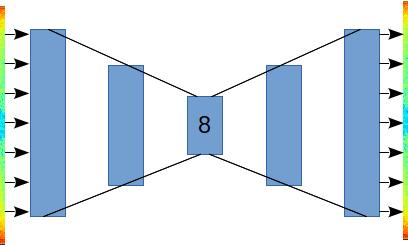
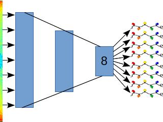
Since the ultimate goal is to light up different Christmas lights at different rhythms in the song, what we need to do is to learn a compressed representation of the audio input at each time step. The spectrogram works perfectly for this. There are 513 frequency ‘features’ at each time step, so the goal of our autoencoder will be to build an 8-channel representation of each time step (To match the number of light channels). Note that this is essentially a dimensionality reduction technique, and the standard set of algorithms could be applied here (PCA and tSNE are my favorite, perhaps we’ll do another post on those¹). Something like this:

We’ll train “A Mad Russian’s Christmas” and test on “Christmas Sarajevo”. First, lets get some setup out of the way:

from spectrogramUtils import * #(Check Bitbucket link for this file. Or use pyplot.specgram....)

import pandas as pd
import numpy as np
from sklearn.preprocessing import MinMaxScaler
from matplotlib import pyplot as plt

from keras.layers import Input, Dense, Dropout

## C:\Users\mj514\ANACON~1\lib\site-packages\h5py\__init__.py:36: FutureWarning: Conversion of the second argument of issubdtype from `float` to `np.floating` is deprecated. In future, it will be treated as `np.float64 == np.dtype(float).type`.
##   from ._conv import register_converters as _register_converters
## Using TensorFlow backend.

from keras.models import Model

Now, create extract the spectrograms out of the the data. Here is a code snippet that will convert your entire music library into .wav (make sure you have ffmpeg installed first) :

import os, re, subprocess
paths = []
for r, d, f in os.walk('C:/Users/mj514/Music/'):
    for file in f:
        if ".mp3" in file:
            strippedFileName = re.sub('[^A-Za-z0-9-mp3]+', '', file.split('.')[0] )#remove special characters and file ending
            strippedFileName = strippedFileName
            paths.append((r + '/' + file,strippedFileName))
    for aTuple in paths:
      subprocess.call(f'ffmpeg -i "{aTuple[0]}" wavs\{aTuple[1]}.wav', shell = True)

The plotstft function (from spectrogramUtils, adapted from here) breaks our song up into frequency components, and returns a .npy array with 513 features and some number of time step features.

madIms = plotstft('C:/Users/mj514/Documents/dataSci/christmasAutoencoder/maddrussian.wav')

christmasSarajevoIms = plotstft('C:/Users/mj514/Documents/dataSci/christmasAutoencoder/christmasSerajevo.wav')

print(f"Class: {madIms.__class__}, shape: {madIms.shape}") # I recently fell in love with fstrings!!!

## Class: <class 'numpy.ndarray'>, shape: (24330, 513)

Here I chose to do min-max scaling, as my input has a predictable amplitude. I build the transformation on the train song (madIms) and apply it to the test song(christmasSarajevoIms)

scaler = MinMaxScaler()
x_train = scaler.fit_transform(madIms) 
x_test = scaler.transform(christmasSarajevoIms)

Next, let’s set up our autoencoder. As you can see the encoder steps progressively down until we get to the desired number of channels, and the decoder steps the input back up to the full 513 output. While the measured loss doesn’t improve significantly with added layers ( you can get the same network performance with only 1 hidden layer) I found that the intermediate features are mutch richer with a full encode-decode stack.

def denseAutoencoder(internalActivation = 'tanh'):
    input_img = Input(shape=(513,))
    input_dropped = Dropout(0.2)(input_img)
    encoded = Dense(128, activation=internalActivation, name = 'encode_128')(input_dropped)
    encoded = Dense(64, activation=internalActivation, name = 'encode_64')(encoded)
    encoded = Dense(32, activation=internalActivation, name = 'encode_32')(encoded)
    encoded = Dense(16, activation=internalActivation, name = 'encode_16')(encoded)
    encoded = Dense(8, activation=internalActivation, name = 'encode_8')(encoded)

    decoded = Dense(16, activation=internalActivation, name = 'decode_16')(encoded)
    decoded = Dense(32, activation=internalActivation, name = 'decode_32')(decoded)
    decoded = Dense(64, activation=internalActivation, name = 'decode_64')(decoded)
    decoded = Dense(128, activation=internalActivation, name = 'decode_128')(decoded)
    decoded = Dense(513, activation='sigmoid', name = 'output')(decoded)

    autoencoderDense = Model(input_img, decoded)
    autoencoderDense.compile(optimizer='adam', loss='mean_squared_error')
    return autoencoderDense
    
autoencoderDense = denseAutoencoder()
autoencoderDense.fit(x_train, x_train,
                epochs=10,
                batch_size=256,
                shuffle=True, #important
                validation_data=(x_test, x_test))

It turns out that for this network, tanh activation was better than relu and sigmoid. I suspect tanh was better than relu in this case because of the inherent non linear nature of sound. Looking at the distribution of magnitudes, there isn’t much of a skew, so maybe I’m wrong:

plt.hist(madIms.flatten(),bins=500)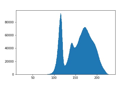

While it can be tempting to assume the default (in this case relu) is the best activation, it’s always best to explore.

Analyze Output

So how well did we do? Lets look at the reconstructed (top) and the original (bottom):

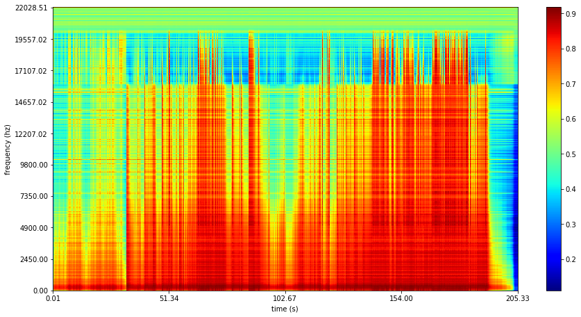
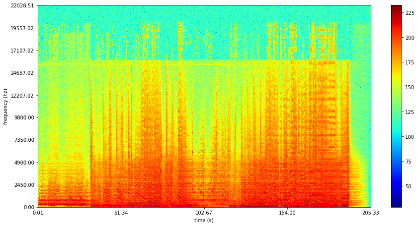
The reconstructed is significantly less noisy (one of the applications for autoencoders), but seems to do a good job capturing the basic structure.

The final step is to clip off the decode layers and get the activations for the intermediate layers:

To do this, we can use the keract package

from keract import get_activations
active = get_activations(autoencoderDense, x_test)
_ = {print(k + str(v.shape)) for k,v in active.items()}

## dropout_1/cond/Merge:0(17686, 513)
## encode_128/Tanh:0(17686, 128)
## encode_64/Tanh:0(17686, 64)
## encode_32/Tanh:0(17686, 32)
## encode_16/Tanh:0(17686, 16)
## encode_8/Tanh:0(17686, 8) # this is the one we want
## decode_16/Tanh:0(17686, 16)
## decode_32/Tanh:0(17686, 32)
## decode_64/Tanh:0(17686, 64)
## decode_128/Tanh:0(17686, 128)
## output/Sigmoid:0(17686, 513)

intermediateLayerName = list(active.keys())[5]

Plotting the activations of the encode_8 layer over time gives:

plt.figure(figsize=(15, 6.5))
plt.plot(active[intermediateLayerName], linewidth=0.1)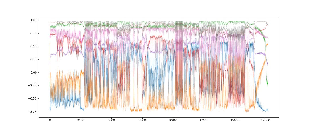

Here is a super zoomed version (you have to click the graph, I promise it’s worth it.)

Conclusion

It turns out, not even Christmas Lights are safe from the oncoming AI revolution! This analysis leaves room for quite a bit of additional exploration:

• Does the reconstruction work well on songs from other artists/in other genres?
• Is there a way to use stereo sound (only used one side of the input here) to improve the reconstruction and thus the quality of the compressed signal?
• What other architectures could be used? (CNN,RNN)
• Can we classify the songs based on artist or genre?
• Can we get it working on the Raspberry Pi?
  

For the next post, we’ll be exploring how to improve the encoding by removing the end bits from the song, allowing the intermediate features to capture a richer representation of the important parts of the song. I’ll also show how we can use a 1D Convolutional Network to build a more accurate reconstruction. Do you have other ideas? Comment below to let me know!