Calculating The Odds

For our simple case, where we can define binary outcomes (boy/girl, heads/tails, pass/fail, etc…), and we’re interested in calculating the probability of an outcome that meets a specified criteria (5 girls out of 5 children), the binomial distribution allows us to calculate this directly.

The binomial distribution is given by:

\(\mathrm{P}(X=k) = \binom{n}{k} p^k(1-p)^{n-k}\)

where \(k\) is equal to the number of success (in this case the number of boys), \(n\) is the number of Bernoulli trials (in this case, the number of children) and \(p\) is the probability of boys or girls (our null hypothesis puts this at 50%). Our case is a simple version of the above, where \(k = n\), and \(p = 1-p = 0.5)\) so the equation above simplifies to:

\(\mathrm{P}(X=k| k = n, p = 0.5) = \ p^k\)

Lets calculate this probability for families with 1-10 children of the same sex, and see where the cutoff is:

library(tidyverse)
data_frame(numChildren = 1:10) %>%
  mutate(probabilityAllBoys = 0.5^numChildren) %>%
  ggplot(aes(numChildren,probabilityAllBoys)) +
  geom_point() + 
  geom_text(aes(label = round(probabilityAllBoys,3)*100),nudge_y = .015,nudge_x = -0.2) + 
  geom_hline(yintercept=.05, linetype="dashed", color = "red") + 
  scale_y_continuous(labels = scales::percent) + 
  ggtitle("Probability That All Children Will be Boys By Family Size")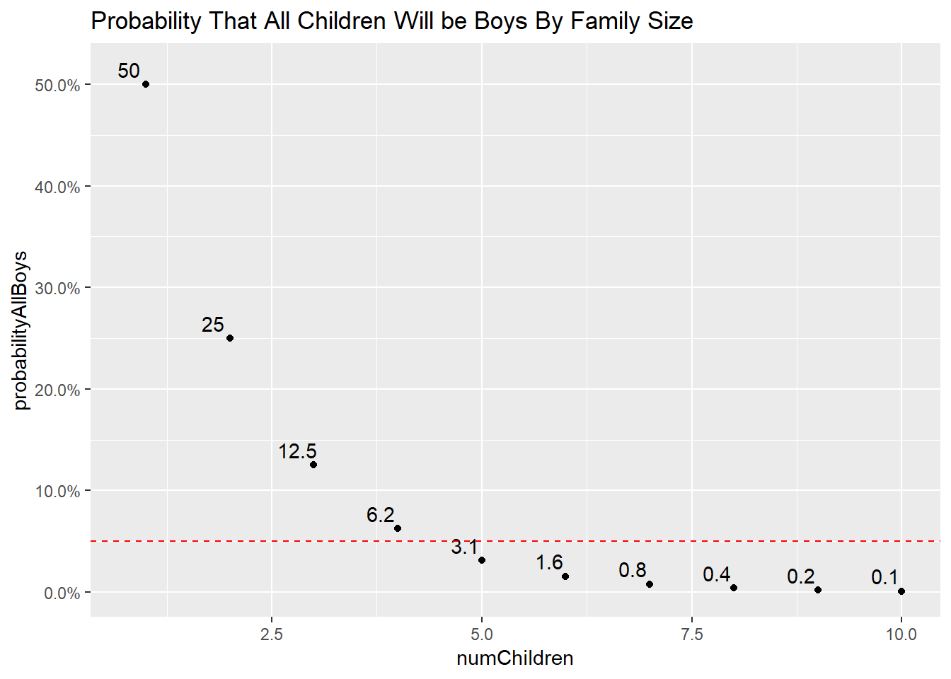

This chart shows that if the probability of boy and girl are equal, and you sampled 100 families with 5 children, you would expect ~3 of the families to have all boys!

Often I encounter problems that are complicated enough that the odds are not directly calculable . In this case we can employ my favorite method for doing hypothesis testing: Simulation.

A Simple Simulation

Lets say we didn’t know (or were too lazy) to calculate the equation above. We could imagine a set of pretend families who had pretend children in a way that aligns to the null hypothesis (50/50 chance of boy/girl), and figure out how often those families had all boys.

100 Families

(OK so this is not a pretend family and they are all the same, but I’m sure you can use your imagination…)
In R we can use sample to draw from 0s or 1s (boy or girl) with equal probability

set.seed(1)
numberOfChildren = 5
probabilityOfboy = 0.5

oneFamily = sample(c(0,1),numberOfChildren,probabilityOfboy) #simulate one family
oneFamily

## [1] 0 0 1 1 0

Our first family with 5 children had two girls (the 0’s), then two boys(the 1’s), then another girl. Our hypothesis just pertains to the number of boys, so we can just take the sum of our family:

sum(oneFamily)

## [1] 2

And we have the number of boys for this family.

To get the p-value from our plot above, we need to do this procedure for 10,000 or so pretend families, and then calculate the percentage of those trials that match our observation (sum to a total of 5).

It turns out R gives us a shortcut to this, allowing us to get the number of boys positive outcomes from successive Bernoulli trials quite easily:

set.seed(1)
numberOfChildren =5
numberOfFamilies = 1
probabilityOfBoy = 0.5
rbinom(n=numberOfFamilies, size = numberOfChildren, prob = probabilityOfBoy)

## [1] 2

The 2 here represents the same 2 that we got when we did sum(oneFamily)… Our first family has 2 boys. Lets do it now for 10,000 families:

set.seed(1)
numberOfChildren =5
numberOfFamilies = 10000
probabilityOfBoy = 0.5
tenkFamilies = rbinom(n=numberOfFamilies, size = numberOfChildren, prob = probabilityOfBoy)
print(paste0("First Family: ", tenkFamilies[1], " Boys, 5010th Family: ", tenkFamilies[5010]," Boys"))

## [1] "First Family: 2 Boys, 5010th Family: 4 Boys"

How often do we get all boys?

mean(tenkFamilies == 5)

## [1] 0.0328

3.2% is close to the number we arrived at above (3.125) but not exactly. There are two reasons for this.

First, because we are simulating randomness, the outcome of any given experiment (in this case 10000 families) will drift around 3.125, but won’t be precisely 3.125. You can reduce the standard error in the estimate by sampling more families (try 100000000), with error going to zero as numberOfFamilies approaches infinity.

Second, even with more samples, there is likely to be some error in our estimate due to the fact that the random number generator on our computer is not ‘truly’ random. It is a reasonable approximation of randomness, but it turns out randomness is not so easy to generate.

The threshold typically held for rejecting the null hypothesis is 5% or 5 families with this observation out of 100 total families. This suggests that if your family with 5 children has only boys, you can statistically reject the null hypothesis and conclude that this result is not due to random chance! You assumed innocence (normal probability), simulated a bunch of outcomes, and found that the observed outcome (5 children, only boys) is sufficiently rare to believe it isn’t due to random chance.

Well, not so fast…

Some Problems With Our Conclusion

While it is nice to have a conclusive line drawn in the sand about statistical significance, there are several problems with this conclusion. First, note that even with random chance, a non-trivial number of families out of 100 are likely to have all girls or all boys. Given the number of families with children, we must expect at least some of them will have children of only one sex. We could consider the entire distribution of families and discover if it deviates from our expectation, but drawing conclusions based on one family seems difficult in this case

It turns out that this issue has importance beyond simple curiosity. A p-value of 0.05 has been used as the standard across many scientific disciplines as a threshold for declaring a finding statistically significant and therefore publishable. Setting the bar too low means that we might not have reproduceable results setting the bar too high means that important results won’t be be published.

It would appear that the evidence is coming out on the side that the 0.05 threshold is too low, and thus, there has been a push recently to lower the threshold for the p-value from 0.05 to 0.005, or 0.5%. Partially derivative did a nice podcast on this, check it out here.

P Hacking

To get a sense of why this may be a problem we can do a simple thought experiment. The scientific process typically goes something like this:

1. Come up with a hypothesis

• X chemical will produce Y result…

2. Design and execute an experiment to test the hypothesis

• X chemical had Y result with p statistical certainty.

3. If the result was successful (p-value<0.05), write a fancy paper to tell other people.

The formulation of the p-value is purposefully skeptical. It says, “OK, your trying to prove that this or that happens. What if nothing really is going on, how many times would we magically arrive at the conclusion you just observed?”. Lets say we wanted to make the argument that the actual ratio of boys/girls for some populations is not 50/50. To do that we decided to study the distribution of children from 100 families. Turns out if you look at enough groups of 100 families, you’d find one that you could use to support your hypothesis:

Lots of Families

In practice, there are several ways to accidentally find that something is statistically significant. For example, you could simply repeat an experiment until a statistically significant finding is observed. More practically, in the course of experimentation, you might be testing hundreds or thousands of hypothesis at once.

Perhaps you want to study what is influencing the defect rate for a particular widget You collect several thousand variables gathered during the manufacturing process and build a statistical model that predicts the defect rate. In a sense, you are performing thousands and thousands of experiments (probability of defect rate given feature 1,2,3).

Because of this, its highly likely that some of the variables will have statistically significant (p<0.05) correlation to the outcome even there is absolutely no correlation!

This stresses why it is important to evaluate the outcome of these types of experiments with a subject matter expert. Is there some physical or process explanation as to why these are correlated? Does this lead you towards another hypothesis you could use to independently verify the result?

How many children do we need to meet the more stringent p-value suggested by the literature?

library(tidyverse)
data_frame(numChildren = 1:10) %>%
  mutate(probabilityAllBoys = 0.5^numChildren) %>%
  ggplot(aes(numChildren,probabilityAllBoys)) +
  geom_point() + 
  geom_text(aes(label = round(probabilityAllBoys,3)*100),nudge_y = .015,nudge_x = -0.2) + 
  geom_hline(yintercept=.005, linetype="dashed", color = "red") + 
  scale_y_continuous(labels = scales::percent) + 
  ggtitle("Probability That All Children Will be Boys By Family Size")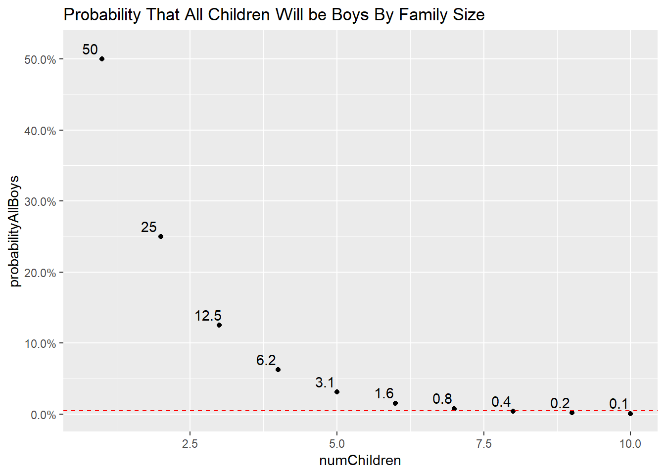

The new, more stringent p-value threshold suggests that if you have 8 children, and they are all one sex, you might have a problem on your hands.

But lets be honest, if you have 8 children, you already have enough to worry about!

But have we formulated the problem properly? What we really care about is how many children would you have to have of either sex to conclude something is wrong. To calculate the probability of this, you double all of the probabilities above. Doing so lands us at 9 children.

If you made it this far, hope you enjoyed reading, and stay tuned for my next blog post which will use the simulation principle developed here to statistically verify claims made in childrens stories with web scraping, nlp, and parallelized simulation.