One of the most interesting talks I heard at Strata in San Francisco this year was “Towards deep and representation learning for talent search at LinkedIn”. In the talk, Gungor explained how he took advantage of LinkedIn’s economic graph to build a hyper-personalized search engine. Ever since then I’ve had graphs firmly planted in my mind.

Not these graphs:

Graph

More like these:

Network

Specifically, I’ve been trying to understand how graph network techniques can be applied in various domains, including natural language processing. Graphs are interesting representations of the world because they capture explicit relationships between items/concepts, allowing an object to be represented in context to all other objects in the graph.

In the LinkedIn example, there are nodes that represent people, skills, location, jobs industries, friends, interactions, and so on. An individual skill or person is then represented with much more context than can be gleaned by just looking at their name.

For example, people who apply machine learning to the telecom industry are similar in some way to people who do machine learning in manufacturing, but the combination of skill + industry + person gives a much better context than just ‘machine learning’ itself.

When the Mueller Report was released and I found that I was way to lazy to read it, I figured I should see if building a graph representation of the document would expedite my understanding of the content, and so here we are.

Building a Graph Representation of The Mueller Report

I wanted to build a graph that would allow me to understand the relationship between different individuals/concepts and also allow me to navigate through the document, following the thread of the story in some intuitive way.

To do this, I decided on the following representation:

Here, each paragraph is represented by a node, and the people, places and things are connected to that paragraph with an edge. While I could have chosen to represent each sentence, I chose paragraph because I wanted a more global representation of the relationships between people.

In this case, people are associated with other people, locations, or concepts if they are mentioned in the same paragraph.

Prepare The Text For Graph Euphoria

In order to construct the graph, we’ll start with extracting the text from the document. Unfortunately the official report was released as a pdf that is simply a collection of images. This introduces some challenges we’ll address later, but first Lets start with stripping the text out of the pdf and splitting on endlines to get something like a bunch of paragraphs:

mueller1 = open('Mueller-Report.pdf', 'rb') 
mueller1Reader = PyPDF2.PdfFileReader(mueller1)

muellerPages = []
for pageNum in range(mueller1Reader.numPages):
    muellerPages.append([par for par in mueller1Reader.getPage(pageNum).extractText().split('\n')])
mueller1.close()

muellerParagraphs = sum(muellerPages,[]) #flatten the list of lists
len(muellerParagraphs)

##897

muellerParagraphs is now a list of all of the ‘paragraphs’ in the Mueller report. Lets take a look at a random paragraph:

to release documents directly to reporters and other interested individuals. Specifically, on June 27, 2016, Guccifer 2.0 sent an email to the news outlet The Smoking Gun offering to provide “exclusive access to some leaked emails linked [to] Hillary Clinton’s staff.”148 The GRU later sent the reporter a password and link to a locked portion of the dcleaks.com website that contained an archive of emails stolen by Unit 26165 from a Clinton Campaign volunteer in March 2016.149 That the Guccifer 2.0…

This paragraph reveals a few things. First, the pdf to text converter works well but not perfectly. Superscripts are captured as normal text with no spaces (the 148 after the " and the 149 after 2016), and there are some pervasive misspellings captured by the tool (Comey is captured as Corney, some words are truncated). You’ll also notice that the paragraph is packed with references to individuals, dates, companies, and locations.

Let’s take a look at how well spaCy does extracting these terms. We’ll first load it and build a ‘THEME’ finder:

nlp = spacy.load('C:/Users/mj514/Anaconda3/lib/site-packages/en_core_web_lg/en_core_web_lg-2.0.0')
terms = (u"collude", u"collusion", 
         u"conspiracy", u"conspire",u"hack", u"hacking", u"cyber intrusions", 
         u"russian hacking", u"hackers",u"social media",u"computer intrusions",
         u"cybersecurity",u"emails","email")
concept_matcher = EntityMatcher(nlp, terms, "THEME")

nlp.add_pipe(concept_matcher, after="ner")

The theme entity matcher simply records any time we see the provided words and references them as a theme. Applying this to our example paragraph and visualizing with the displacy tool shows what we can extract:

from spacy import displacy

aDoc = nlpParagraphs[105]

displacy.serve(aDoc, style="ent")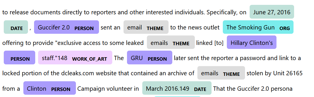

Displacy spaCy does an excellent job picking out the basic features of the text, even recognizing the use of Guccifer 2.0 as a person, but it isn’t perfect. staff.148 is picked up as a work of art. while March 2016 is identified correctly as a date, the entity text extracted includes the period and a reference to the footnote (2016.149). Also, despite being an organization, Unit 26165 isn’t picked up as an entity. Finally, GRU is sometimes referenced to be a person, other times referenced to be an organization.

We’ll focus on GPE, person, and theme, iterating through our paragraphs and creating a node for each paragraph, then attaching the GPE’s, Persons, and Theme’s mentioned in that paragraph with an edge. This is accomplished with the makeGraphFromSpacy function:

fullMuellerG = makeGraphFromSpacy(nlpParagraphs)
pyvisG = Network("1000px", "1000px")
from_nx(pyvisG,fullMuellerG)
pyvisG.show_buttons(filter_=['physics'])
pyvisG.show('fullMueller.html')

And now we have it, the full graph: 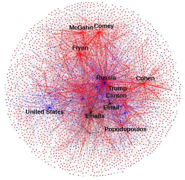Full Mueller Graph

If you are patient, you can check out the full interactive graph here where you can zoom, drag and change the visualization settings (takes about 1 minute to load). If you’re interested in the details behind the makeGraphFromSpacy function checkout my github.

Analyzing The Graph

At first glance, the graph has captured quite a bite of intuitive structure about the document. The people and places that are at the center of the investigation (Trump, Russia, Clinton) are all tightly grouped at the center of the document while Comey, McGahn and Cohen show up near the periphery. Smaller players in the story are hovering around the very outside of the graph making the outside a fun place to find somewhat random subjects.

Paragraph 69 is an example listing fake social media accounts which purported to have connection to real organizations (like the Tennessee Republican Party):

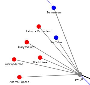
Paragraph 69

For example, one IRA-controlled Twitter account, @TEN_ GOP, purported to be connected to the Tennessee Republican Party.46 More commonly, the IRA created accounts in the names of fictitious U.S. organizations and grassroots groups and used these accounts to pose as immigration groups, Tea Party activists, Black Lives Matter protestors, and other U.S. social and political activists…

Graph Algorithms

One of the most compelling reasons to structure your problem as a graph network problem is the well researched and robust set of graph algorithms available to leverage for exploration and feature construction.

For a clear use case of this approach, take a look at this post where the authors demonstrate a method for predicting future co-authors by using only features generated from a graph. In this case the graph doesn’t capture the area of expertise, key words or terms used in papers, or which journals they are in. Instead, they build an accurate predictor of next coauthor simply by extracting features from a graph representing historical coauthorship.

Lets apply a few algorithms to our Mueller report graph and see what intuition we can gain from it:

pgRank = networkx.algorithms.pagerank(fullMuellerG)
betweenness = networkx.algorithms.betweenness_centrality(fullMuellerG)
closeness = networkx.algorithms.closeness_centrality(fullMuellerG)

rankings = pd.concat([pd.DataFrame([pgRank]).T,pd.DataFrame([betweenness]).T, pd.DataFrame([closeness]).T],axis = 1)
rankings.columns = ['pgRank','betweenness','closeness']
rankings.sort_values('pgRank', ascending = False).head(20).round(4)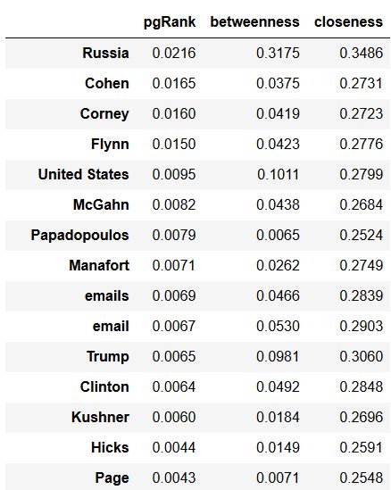

Graph Elements Sorted by PageRank

While I don’t have the space in this blog post to explain these algorithms in detail we can develop get an intuitive understanding for what they are doing.

The PageRank algorithm attempts to identify how important a page is by allowing other pages to ‘vote’ for it. These votes come in the form of links, so naturally pages with more links are considered more important. In this case, the PageRank does a good job identifying the key concepts (those with the most mentions across articles) and ranking them higher. Because our graph is structured where links always go ‘out’ from paragraphs (a paragraph mentions a person, a person doesn’t mention a paragraph) the page rank algorithm more or less judges on the degree of each node (how many connections it has).

The closeness centrality algorithm, which attempts to identify nodes in the network that control and acquire most of information flow throughout the network, tells a very different story: Sorted by closeness Centrality

In this case Trump and Russia (The two concepts that connect nearly the whole document) are pinned to the top, and a set of key paragraphs follow. Paragraph 38 is titled “The Special Counsel’s Charging Decisions” which is likely the most important section in the document for understanding the context and the final outcome. Paragraph 394 contains some of the testimony from both Michael Cohen and Michael Flynn, and paragraph 251 focuses in on the discussion surrounding the meeting at Trump Tower.

Graph Traversal

While these algorithms can give a high level view of the important themes/concepts in the document, lets zoom in on one individual and see what their second order connections look like (It’s interactive, zoom, grab, explore away):

parExample = getSecondOrderSubgraph(G,'Ivanka Trump')
ivankaViz = Network("500px", "500px")
from_nx(ivankaViz,parExample)
ivankaViz.show('Ivanka.html')

This view shows all of the paragraphs Ivanka Trump’s mentioned in (only 3) and all of the people/places and things that are mentioned alongside those paragraphs. From here you can see that two of the paragraphs mentioned Russia, all 3 deal with emails, and several mention Hope Hicks.

Doing something similar with Kellyanne Conway shows that she is only mentioned in 2 paragraphs, both of which mention Steve Bannon:

While this is an interesting way to view and navigate the document, it tends to produce some overwhelming visuals viewing very well connected nodes Here is the 2nd order graph for James Comey in case you don’t believe me: Comey Subgraph

Building a Paragraph Reccomender Engine

Lets combine the ability to identify relevant/important articles using centrality algorithms with our graph traversal system to produce a recommend engine for paragraphs you might want to read concerning a specific topic.

First, we build a paragraphDataframe that will be helpful in displaying the results.

paragraphDF = pd.DataFrame({'text':muellerParagraphs,'paragraph':[f'par_{num}' for num in range(len(muellerParagraphs))]})
paragraphDF['paragraph'] = paragraphDF.paragraph.astype('str') # Because pandas is stupid

for one reason or another Pandas makes the decision to encode our list of strings into a generic ‘object’, which proves difficult when joining with the following step, so we’ll change the metadata to string.

Then we can define our whatToRead function which takes our search concept and our full graph, finds the n = 2 subgraph of connections, determines the closeness centrality, and joins with the paragraph dataframe to be able to display the results:

def whatToRead(concept, fullGraph, topn = 10):
    subGraph = getSecondOrderSubgraph(fullGraph,concept)
    betweenness = networkx.algorithms.closeness_centrality(subGraph)
    readDF = pd.DataFrame([betweenness]).T.sort_values(0, ascending=False).head(topn)
    readDF.reset_index(inplace=True)
    readDF.columns = ['paragraph','score']
    print(readDF)

    matchingParagraphs = readDF.merge(paragraphDF,on = 'paragraph', how = 'inner')
    return matchingParagraphs

Lets try it out on James Comey and see what comes out:

toRead = whatToRead('Corney',fullMuellerG)

## Nodes: 418
## Edges: 817
## Self Loops: 0
##      index         0
## 0  Corney   0.596572
## 1  Russia   0.137260
## 2  McGahn   0.071890
## 3  par_461  0.063138
## 4  par_517  0.059846
## 5  par_648  0.050754
## 6  Flynn    0.044999
## 7  par_650  0.044556
## 8  par_521  0.040857
## 9  par_464  0.039705

The items in the subgraph with the most betweenness are Comey himself (remember the text parser misspells his name…), Russia, and McGahn who served as White House Council through most of the investigation. Paragraph 461 is an interesting one, here is an excerpt:

On January 26, 2017, Department of Justice (DOJ) officials notified the White House that Flynn and the Russian Ambassador had discussed sanctions and that Flynn had been interviewed by the FBT. The next night, the President had a private dinner with FBI Director James Corney in which he asked for Corney’s loyalty. On February 13, 2017, the President asked Flynn to resign. The following day, the President had a one-on-one conversation with Corney in which he said, “I hope you can see your way clear to letting this go, to letting Flynn go.”

As you can see our paragraph recommender managed to grab a paragraph that discusses the key elements of the investigation surrounding James Comey and the presidents motivation for removing him from his position as the Director of the FBI.

Looking further down the list, paragraph 517 discusses how James Comey confirmed the existence of the Russia investigation, and paragraph 648 discusses Trump’s anger at the way James Comey handled the Clinton email investigation.

While it’s difficult to show empirically that these are the most important paragraphs to read about the part James Comey played in the investigation, it’s clear the algorithm has picked out paragraphs that highlight some of the key events surrounding the involvement of Comey in the whole plot line.

What Sucks and What’s Next

While there is certainly some promise in applying graph techniques and algorithms to articles like this one, this analysis isn’t without it’s drawbacks and area’s of improvements.

There are several things that would make this analysis quite a bit cleaner:

Correcting up the parsing errors.
Deduplicating the names of entities (Donald Trump = Donald J Trump = Trump)
Building a custom NER model for the special entities in the text (Democratic National Convention, hacking groups, concepts)

The same strategy applied for the paragraphs of this single document could be used to explore an entire corpus of documents. For example, leveraging the references in academic papers as well as the language used in the abstract could be used to find the best papers to read on a given topic.

Finally, a key element of the advantage of a graph network is to build distributed representations of the nodes of the graph that are able to capture context and use it for clustering and machine learning. I’ve got a follow up blog post that will do just that, using only 14 lines of python code. If you’re interested in a sneak peek, feel free to check out my github linked below.

As always, if you have any comments, ideas for improvement, or things you’d like to see me write a blog about, leave a comment below!

nlp spacy graph trump mueller python visualization pyvis networkx

Graph Visualization of The Mueller Report With SpaCy and PyVis

Building a contextual paragraph recomendation engine